Simulate dToF Sensors
The dtof module of the sensors subpackage provides implementations for multiple dToF SPC cameras, allowing users to choose how the SPC data is captured and processed. In this tutorial we will explore three major types of SPC sensor classes.
Simulate RawSPC
The camera simulated using RawSPC class generates photon cube of raw timestamps. We use the PerPixelLoader class to simulate different scene distances and illumination conditions.
[ ]:
from SPCSim.data_loaders.perpixel_loaders import PerPixelLoader
from SPCSim.data_loaders.transient_loaders import TransientGenerator
from SPCSim.utils.plot_utils import plot_transient
import matplotlib.pyplot as plt
from SPCSim.sensors.dtof import RawSPC
import torch
import numpy as np


# Simulating results for distance = 0.1*dmax
PixLdr = PerPixelLoader(
                        num_dists=5,
                        min_dist = 0.2,
                        max_dist = 0.8,
                        tmax = 100,
                        sig_bkg_list = [
                            [0.2,0.2]],
                        num_runs=5,
                        device = "cpu")

# Generate the per pixel data
data = PixLdr.get_data()


# Creating transient generator with laser time period of 100ns, FWHM 1 and with
# laser time period divided into 1000 equal time-bins
tr_gen = TransientGenerator(Nr = PixLdr.Nr, Nc = PixLdr.Nc, N_tbins = 1000, tmax = PixLdr.tmax, FWHM = 2)


# Using the get function to generate the transient
# for a given distance, albedo, intensity, and illumination condition
phi_bar = tr_gen.get_transient(data["gt_dist"],
                               data["albedo"],
                               data["albedo"],
                               data["alpha_sig"],
                               data["alpha_bkg"])

Nr, Nc, N_tbins = phi_bar.shape
device = PixLdr.device
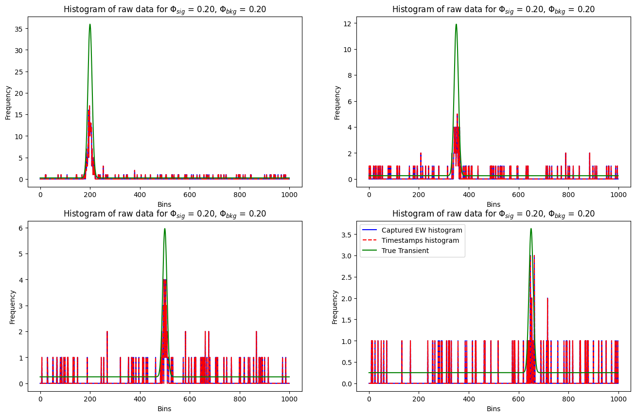
The capture method returns the raw_data and corresponding equi-width histogram data. The raw_data is a 3D tensor of shape (Nr,Nc,N_output_ts) where N_output_ts is the number of output timestamps per pixels.
Note: To support vectorized computations the current implementation of RawSPC assumes one time stamp vector per laser cycle and returns 0 if no timestamp is detected for a laser cycle. (Hence N_pulses = N_output_ts)
[ ]:
N_output_ts = 500
N_pulses = 400

# Creating the RawSPC object with desired intrinsic properties
spc1 = RawSPC(Nr,
              Nc,
              N_pulses,
              device,
              N_tbins,
              N_output_ts)

# Captured data contains timestamps (Nr x Nc x N_output_ts) and ewh (Nr x Nc x N_tbins)
captured_data = spc1.capture(phi_bar)

# Accessing the timestamp data
raw_data = captured_data["time_stamps"]

# Accessing the corresponding ewh
ewh_data = captured_data["ewh"]
100%|██████████| 400/400 [00:00<00:00, 1028.28it/s]
The capture method returns a dictionary containing the raw timestamps and the captured equi-width histogram. The raw timestamps are passed to torch.histogram to create an equi-width histogram. The overlapping blue and red graphs indicate that N_output_ts is large enough to store all the time stamps detected by the camera for the complete exposure time. (Try playing with different combinations of background or signal flux or the number of laser cycles for better understanding)
[7]:
print("raw_data", raw_data.shape, raw_data.min(), raw_data.max())
fig, ax = plt.subplots(2,2,figsize=(16,10))
xaxis = torch.arange(0.5,1+N_tbins).to(torch.float)
print(xaxis.shape, xaxis)


# For first distance value and second run
ROW = PixLdr.get_row(sbr_idx =0, dist_idx=0)
RUN = 2
hist,_ = torch.histogram(raw_data[ROW,RUN,:], xaxis)
hist2 = ewh_data[ROW,RUN,:]
plot_transient(ax[0,0], hist2.cpu().numpy(), plt_type = '-b', label="Captured EW histogram")
plot_transient(ax[0,0], hist.cpu().numpy(), plt_type = '--r', label="Timestamps histogram")
plot_transient(ax[0,0], phi_bar[ROW,RUN,:].cpu().numpy()*spc1.N_output_ts/np.mean(np.sum(phi_bar.cpu().numpy(), axis=-1)), plt_type = '-g', label="True Transient")
ax[0,0].set_xlabel('Bins')
ax[0,0].set_ylabel('Frequency')
ax[0,0].set_title(r'Histogram of raw data for $\Phi_{sig}$ = %.2f, $\Phi_{bkg}$ = %.2f'%(data["alpha_sig"][ROW, RUN], data["alpha_bkg"][ROW, RUN]))

# For second distance value and second run
ROW = PixLdr.get_row(sbr_idx =0, dist_idx=1)
RUN = 2
hist,_ = torch.histogram(raw_data[ROW,RUN,:], xaxis)
hist2 = ewh_data[ROW,RUN,:]
plot_transient(ax[0,1], hist2.cpu().numpy(), plt_type = '-b', label="Captured EW histogram")
plot_transient(ax[0,1], hist.cpu().numpy(), plt_type = '--r', label="Timestamps histogram")
plot_transient(ax[0,1], phi_bar[ROW,RUN,:].cpu().numpy()*spc1.N_output_ts/np.mean(np.sum(phi_bar.cpu().numpy(), axis=-1)), plt_type = '-g', label="True Transient")
ax[0,1].set_xlabel('Bins')
ax[0,1].set_ylabel('Frequency')
ax[0,1].set_title(r'Histogram of raw data for $\Phi_{sig}$ = %.2f, $\Phi_{bkg}$ = %.2f'%(data["alpha_sig"][ROW, RUN], data["alpha_bkg"][ROW, RUN]))

# For third distance value and second run
ROW = PixLdr.get_row(sbr_idx =0, dist_idx=2)
RUN = 2
hist,_ = torch.histogram(raw_data[ROW,RUN,:], xaxis)
hist2 = ewh_data[ROW,RUN,:]
plot_transient(ax[1,0], hist2.cpu().numpy(), plt_type = '-b', label="Captured EW histogram")
plot_transient(ax[1,0], hist.cpu().numpy(), plt_type = '--r', label="Timestamps histogram")
plot_transient(ax[1,0], phi_bar[ROW,RUN,:].cpu().numpy()*spc1.N_output_ts/np.mean(np.sum(phi_bar.cpu().numpy(), axis=-1)), plt_type = '-g', label="True Transient")
ax[1,0].set_xlabel('Bins')
ax[1,0].set_ylabel('Frequency')
ax[1,0].set_title(r'Histogram of raw data for $\Phi_{sig}$ = %.2f, $\Phi_{bkg}$ = %.2f'%(data["alpha_sig"][ROW, RUN], data["alpha_bkg"][ROW, RUN]))

# For fourth distance value and second run
ROW = PixLdr.get_row(sbr_idx =0, dist_idx=3)
RUN = 2
hist,_ = torch.histogram(raw_data[ROW,RUN,:], xaxis)
hist2 = ewh_data[ROW,RUN,:]
plot_transient(ax[1,1], hist2.cpu().numpy(), plt_type = '-b', label="Captured EW histogram")
plot_transient(ax[1,1], hist.cpu().numpy(), plt_type = '--r', label="Timestamps histogram")
plot_transient(ax[1,1], phi_bar[ROW,RUN,:].cpu().numpy()*spc1.N_output_ts/np.mean(np.sum(phi_bar.cpu().numpy(), axis=-1)), plt_type = '-g', label="True Transient")
ax[1,1].set_xlabel('Bins')
ax[1,1].set_ylabel('Frequency')
ax[1,1].set_title(r'Histogram of raw data for $\Phi_{sig}$ = %.2f, $\Phi_{bkg}$ = %.2f'%(data["alpha_sig"][ROW, RUN], data["alpha_bkg"][ROW, RUN]))
# ax[3].set_ylim(0, N_output_ts*0.2*(PixLdr.sig_bkg_list[0][0] + PixLdr.sig_bkg_list[0][1]))
plt.legend()
plt.show()
raw_data torch.Size([5, 5, 500]) tensor(0.) tensor(998.5000)
torch.Size([1001]) tensor([5.0000e-01, 1.5000e+00, 2.5000e+00,  ..., 9.9850e+02, 9.9950e+02,
        1.0005e+03])
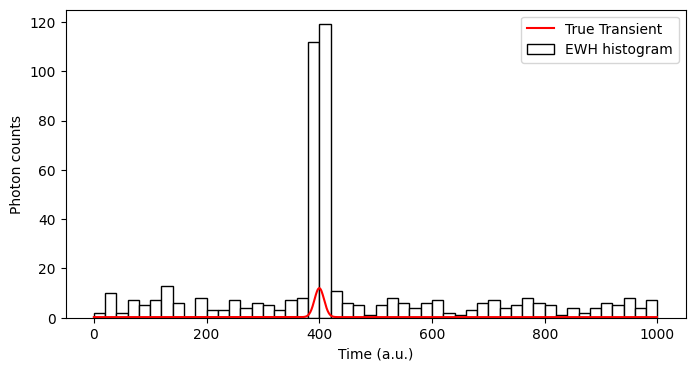
Simulate EWHSPC
The BaseEWHSPC class to simulate the conventional 3D SPCs that compress the photon timestamps into equi-width histograms. The overall pixel processing pipeline is called equi-width histogrammer (EWH).
[50]:
from SPCSim.sensors import BaseEWHSPC
from SPCSim.utils import plot_transient, plot_ewh


# Simulating results for distance = 0.1*dmax
PixLdr = PerPixelLoader(min_dist = 0.4,
                        tmax = 100,
                        sig_bkg_list = [
                            [0.5,0.5]],
                        device = "cpu")

# Generate the per pixel data
data = PixLdr.get_data()


# Creating transient generator with laser time period of 100ns, FWHM 1 and with
# laser time period divided into 1000 equal time-bins
tr_gen = TransientGenerator(N_tbins = 1000, tmax = PixLdr.tmax, FWHM = 2)


# Using the get function to generate the transient
# for a given distance, albedo, intensity, and illumination condition
phi_bar = tr_gen.get_transient(data["gt_dist"],
                               data["albedo"],
                               data["albedo"],
                               data["alpha_sig"],
                               data["alpha_bkg"])


# Setting the dimensions, device, number of EWH bins per pixel
# and number of laser pulses

Nr, Nc, N_tbins = phi_bar.shape
device = PixLdr.device
[51]:
N_ewhbins = 50
N_pulses = 500

spc1 = BaseEWHSPC(
                Nr,
                Nc,
                N_pulses,
                device,
                N_tbins,
                N_ewhbins
               )

captured_data = spc1.capture(phi_bar)
ewh_data = captured_data["ewh"].cpu().numpy()
phi_bar = phi_bar.cpu()

ewh_bins_axis = torch.linspace(0,N_tbins-N_tbins//N_ewhbins,N_ewhbins)

fig, ax = plt.subplots(1,1,figsize=(8,4))
ROW, COL = [0,0]
plot_ewh(ax, ewh_bins_axis, ewh_data[ROW, COL,:], label = "EWH histogram", color = 'w')
plot_transient(ax, phi_bar[ROW, COL,:].numpy()*spc1.N_pulses, plt_type = '-r', label="True Transient")
ax.set_xlabel("Time (a.u.)")
ax.set_ylabel("Photon counts")
plt.legend()
# fig.savefig("Temp.png")
100%|██████████| 500/500 [00:00<00:00, 5051.02it/s]
[51]:
<matplotlib.legend.Legend at 0x7d86a08875e0>
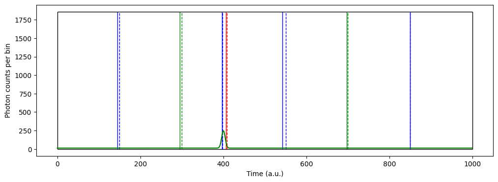
Simulate basic EDH SPCs
The BaseEDHSPC class simulates the oracle equi-depth histogrammer (Oracle EDH). The oracle EDH has access to all the timestamps.
[62]:
from SPCSim.sensors import BaseEDHSPC
from SPCSim.utils import plot_transient, plot_ewh, plot_edh


# Using the get function to generate the transient
# for a given distance, albedo, intensity, and illumination condition
phi_bar = tr_gen.get_transient(
                                data["gt_dist"],
                                data["albedo"],
                                data["albedo"],
                                data["alpha_sig"],
                                data["alpha_bkg"])


# Setting the dimensions, device, number of EWH bins per pixel
# and number of laser pulses

Nr, Nc, N_tbins = phi_bar.shape
device = PixLdr.device
N_edhbins = 8
N_pulses = 5000

spc1 = BaseEDHSPC(Nr,
              Nc,
              N_pulses,
              device,
              N_tbins,
              N_edhbins)

captured_data = spc1.capture(phi_bar)
oedh_data = captured_data["oedh"]
gtedh_data = captured_data["gtedh"]

ewh_data = captured_data["ewh"]
fig, ax = plt.subplots(1,1, figsize=(12,4))

ROW, COL = [0,0]

ymax = ((torch.sum(ewh_data[ROW,COL,:])/N_edhbins)).item()

plot_edh(oedh_data[ROW,COL,:],
         ax,
         ymax = ymax)

plot_edh(gtedh_data[ROW,COL,:], ax,
         tr = phi_bar[ROW, COL,:].numpy()*spc1.N_pulses,
        #  crop_window= tr_gen.FWHM*1.5*tr_gen.N_tbins*1.0/tr_gen.tmax, # uncoment this line to zoom into peak
         ymax = ymax, ls='--')
100%|██████████| 5000/5000 [00:00<00:00, 8819.14it/s]
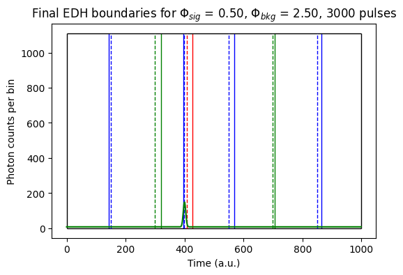
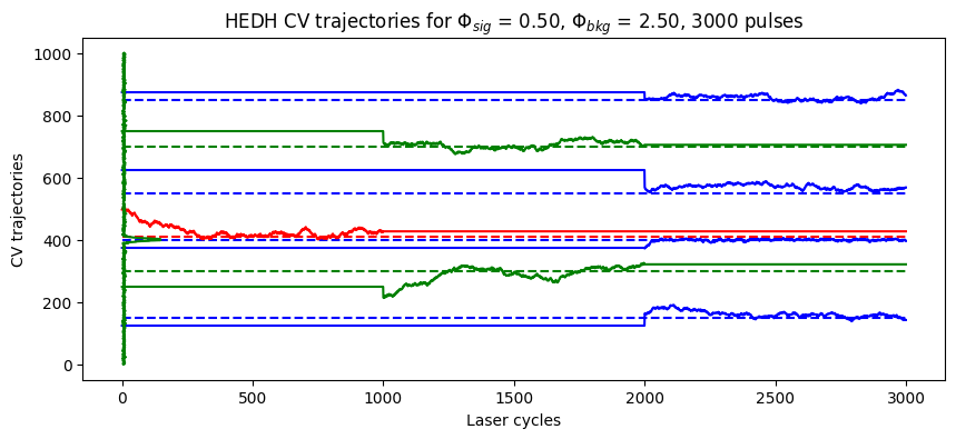
Simulate hierarchical EDH SPCs
The oracle EDH is not memory efficient. Hierarchical ED histogrammers (HEDH) [1] use binner circuits to iteratively update the estimates for ED histogram boundaries.
[68]:
from SPCSim.sensors import HEDHBaseClass
from SPCSim.utils import plot_transient, plot_edh, plot_edh_traj


phi_bar = tr_gen.get_transient(data["gt_dist"],
                               data["albedo"],
                               data["albedo"],
                               data["alpha_sig"],
                               data["alpha_bkg"])


# Setting the dimensions, device, number of EWH bins per pixel
# and number of laser pulses

Nr, Nc, N_tbins = phi_bar.shape
device = PixLdr.device
N_edhbins = 8
N_pulses = 3000

spc1 = HEDHBaseClass(Nr,
              Nc,
              N_pulses,
              device,
              N_tbins,
              N_edhbins,
              step_params={
                  "k":2,
                  "step_vals":[1],
              })

captured_data = spc1.capture(phi_bar)

pedh_data = captured_data["edh"]
gtedh_data = captured_data["gtedh"]
ewh_data = captured_data["ewh"]
edh_list = captured_data["traj"]
edh_list = np.array(edh_list)

ROW, COL = [0,0]

fig, ax = plt.subplots(1,1, figsize=(6,4))
ymax = ((torch.sum(ewh_data[ROW,COL,:])/N_edhbins)).item()
plot_edh(pedh_data[ROW,COL,:].cpu().numpy(),
         ax,
         ymax = ymax)
plot_edh(gtedh_data[ROW,COL,:].cpu().numpy(), ax,
         tr = phi_bar[ROW, COL,:].numpy()*spc1.N_pulses,
        #  crop_window= tr_gen.FWHM*1.5*tr_gen.N_tbins*1.0/tr_gen.tmax,
         ymax = ymax, ls='--')
ax.set_title(r'Final EDH boundaries for $\Phi_{sig}$ = %.2f, $\Phi_{bkg}$ = %.2f, %d pulses'%(data["alpha_sig"][ROW,COL], data["alpha_bkg"][ROW,COL], spc1.N_pulses))
# fig.savefig("Temp.png")

fig1, ax1 = plt.subplots(1,1, figsize=(10,4))
plot_edh_traj(ax1, edh_list, gtedh_data[ROW,COL,1:-1], ewh_data[0,0,:].cpu().numpy())
ax1.set_title(r'HEDH CV trajectories for $\Phi_{sig}$ = %.2f, $\Phi_{bkg}$ = %.2f, %d pulses'%(data["alpha_sig"][ROW,COL], data["alpha_bkg"][ROW,COL], spc1.N_pulses))
# fig1.savefig("TempTraj.png")
3000
100%|██████████| 3000/3000 [00:08<00:00, 374.34it/s]
(3000, 7)
torch.Size([7])
[68]:
Text(0.5, 1.0, 'HEDH CV trajectories for $\\Phi_{sig}$ = 0.50, $\\Phi_{bkg}$ = 2.50, 3000 pulses')
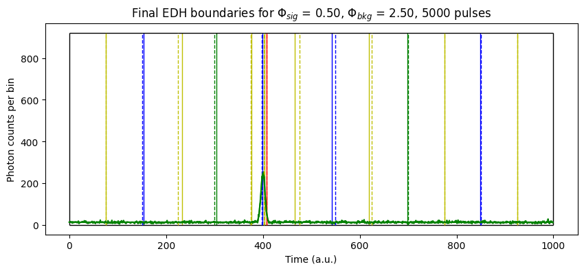
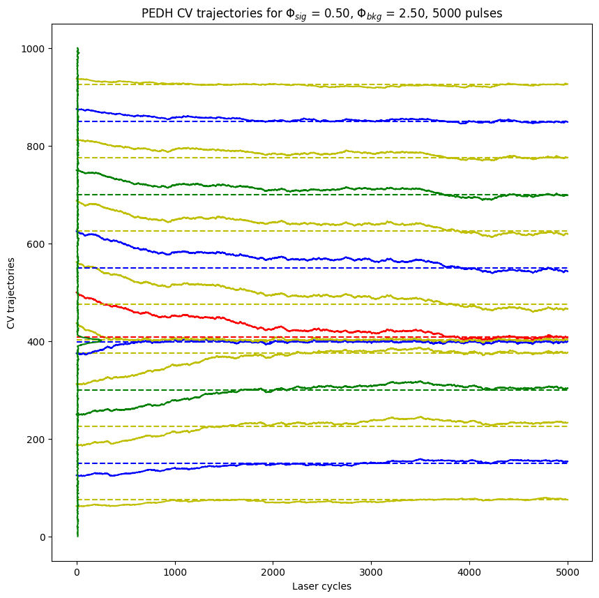
Simulate proportional EDH SPCs
The PEDHBaseClass simulates the proportional ED histogrammers [2]. PEDH uses a proportional binner circuit to track the ED histogram boundaries without storing the photon timestamps.
[69]:
from SPCSim.sensors import PEDHBaseClass
from SPCSim.utils import plot_transient, plot_edh, plot_edh_traj

# Generate the per pixel data
data = PixLdr.get_data()

# Creating transient generator with laser time period of 100ns, FWHM 1 and with
# laser time period divided into 1000 equal time-bins
tr_gen = TransientGenerator(N_tbins = 1000, tmax = PixLdr.tmax, FWHM = 1)


# Using the get function to generate the transient
# for a given distance, albedo, intensity, and illumination condition
phi_bar = tr_gen.get_transient(data["gt_dist"],
                               data["albedo"],
                               data["albedo"],
                               data["alpha_sig"],
                               data["alpha_bkg"])
[70]:
# Setting the dimensions, device, number of EWH bins per pixel
# and number of laser pulses
Nr, Nc, N_tbins = phi_bar.shape
device = PixLdr.device
N_edhbins = 16
N_pulses = 5000
print(N_pulses)

spc1 = PEDHBaseClass(Nr,
              Nc,
              N_pulses,
              device,
              N_tbins,
              N_edhbins,
              step_params={
                  "k":1
              })

captured_data = spc1.capture(phi_bar)

pedh_data = captured_data["edh"]
gtedh_data = captured_data["gtedh"]
ewh_data = captured_data["ewh"]
edh_list = captured_data["traj"]
edh_list = np.array(edh_list)
5000
100%|██████████| 5000/5000 [00:13<00:00, 378.76it/s]
[71]:
ROW, COL = [0,0]

fig, ax = plt.subplots(1,1, figsize=(10,4))
ymax = ((torch.sum(ewh_data[ROW,COL,:])/N_edhbins)).item()
plot_edh(pedh_data[ROW,COL,:],
         ax,
         tr = ewh_data[ROW, COL,:].numpy(),
         ymax = ymax)
plot_edh(gtedh_data[ROW,COL,:], ax,
         tr = phi_bar[ROW, COL,:].numpy()*spc1.N_pulses,
        #  crop_window= tr_gen.FWHM*1.5*tr_gen.N_tbins*1.0/tr_gen.tmax,
         ymax = ymax, ls='--')
ax.set_title(r'Final EDH boundaries for $\Phi_{sig}$ = %.2f, $\Phi_{bkg}$ = %.2f, %d pulses'%(data["alpha_sig"][ROW,COL], data["alpha_bkg"][ROW,COL], spc1.N_pulses))

fig1, ax1 = plt.subplots(1,1, figsize=(10,10))
plot_edh_traj(ax1, edh_list, gtedh_data[ROW,COL,1:-1], ewh_data[0,0,:].cpu().numpy())
ax1.set_title(r'PEDH CV trajectories for $\Phi_{sig}$ = %.2f, $\Phi_{bkg}$ = %.2f, %d pulses'%(data["alpha_sig"][ROW,COL], data["alpha_bkg"][ROW,COL], spc1.N_pulses))
(5000, 15)
torch.Size([15])
[71]:
Text(0.5, 1.0, 'PEDH CV trajectories for $\\Phi_{sig}$ = 0.50, $\\Phi_{bkg}$ = 2.50, 5000 pulses')
References **********
[1] A. Ingle and D. Maier, “Count-Free Single-Photon 3D Imaging with Race Logic,” in IEEE Transactions on Pattern Analysis and Machine Intelligence, doi: 10.1109/TPAMI.2023.3302822,
[2] Sadekar, K., Maier, D., & Ingle, A. (2025). Single-Photon 3D Imaging with Equi-Depth Photon Histograms. In European Conference on Computer Vision (pp. 381-398). Springer, Cham.